Generative AI and diffusion models
Jun 7, 2025
We build a U-Net capable of generating images from pure noise, refine image quality using the diffusion denoising process, guide image creation through context embeddings, and ultimately generate images from English text prompts using the CLIP (Contrastive Language–Image Pretraining) neural network. Based on materials from the NVIDIA Deep Learning Institute’s course on Generative AI with Diffusion Models, Chenyang Yuan’s smalldiffusion (blog), and the excellent stepwise guide by Nakkiran et al. (2024).
Data
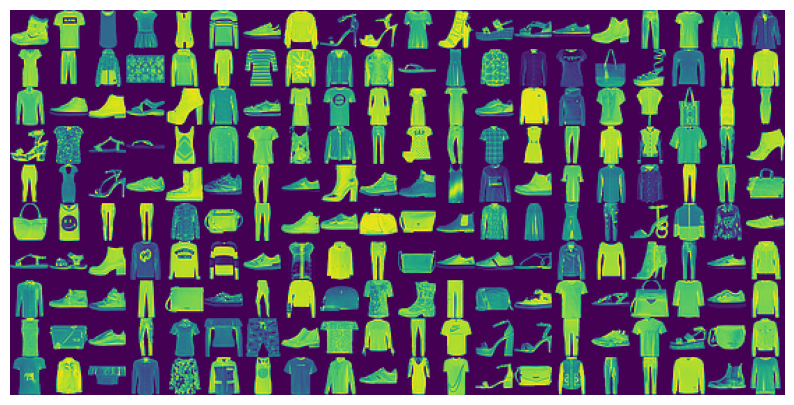
train_set = torchvision.datasets.FashionMNIST(
    "./data/", download=True, transform=transforms.Compose([transforms.ToTensor()])
)
| Dimension | Meaning | Example |
|---|---|---|
| B (Batch) | Number of samples processed together | 32 images in one training step |
| C (Channels) | Feature maps or color channels | RGB = 3 channels; CNN layers = many |
| H (Height) | Image/feature map vertical dimension | 64 pixels tall |
| W (Width) | Image/feature map horizontal dimension | 64 pixels wide |
| Normalization | Normalizes Over | Meaning |
|---|---|---|
| BatchNorm | B, H, W | One channel uses statistics from whole batch + pixels |
| LayerNorm | C, H, W | Entire sample normalized as one vector |
| InstanceNorm | H, W | Each channel of each sample normalized alone |
| GroupNorm | Cgroup, H, W | Channels split into groups; each group normalized |
When training a neural network, the values flowing through the layers can change their scale or distribution as the model updates its weights. This drifting of activations—often called internal covariate shift—can slow down training or cause instability. Batch normalization fixes this by keeping the activations in a stable range.
| Method | Keeps Info? | Learnable? | Notes |
|---|---|---|---|
| Max Pooling | Keeps strongest value only | No | Good for edges, strong signals |
| Avg Pooling | Keeps smooth info | No | Less aggressive |
| Strided Conv | Learns what to keep | Yes | Most popular replacement |
| Adaptive Pooling | Depends | No | Useful for fixed output size |
| Interpolation downsampling | Removes high-freq info | No | Very stable / predictable |
| Blur Pooling | Keeps important info | No | Anti-aliasing |
| Space-to-Depth | Keeps all info | Rearrangement | Lossless downsampling |
MaxPool2d looks at the input feature map in small regions—often 2×2 squares—and selects the single largest number from each region. It then uses these maximum values to create a smaller, condensed version of the feature map. By doing this, the operation reduces the height and width while keeping the most prominent or “strongest” activations. This process helps the network focus on the most important features, such as edges or textures, while reducing memory use and computation. It also provides a small amount of translation invariance, meaning that the network becomes less sensitive to small shifts in the input image.
Denoise with U-Net
You can think of U-Net as having two main phases: compressing the image to understand it, and then rebuilding the image while keeping the details.Ronneberger, Olaf, Philipp Fischer, and Thomas Brox. 2015. “U-Net: Convolutional Networks for Biomedical Image Segmentation.” arXiv:1505.04597
On the left side of the “U” is the encoder (DownBlock). The encoder takes the input image and gradually makes it smaller in height and width while increasing the number of feature channels. At each stage, it uses convolution layers to detect patterns like edges, textures, and shapes, and then uses something like pooling or strided convolutions to downsample. As you go deeper into the encoder, the network stops caring about exact pixel locations and focuses more on what is in the image: for example, that there is a cat, a table, or background.
class DownBlock(nn.Module):
    def __init__(self, in_ch, out_ch):
        kernel_size = 3
        stride = 1
        padding = 1

        super().__init__()
        layers = [
            nn.Conv2d(in_ch, out_ch, kernel_size, stride, padding),
            nn.BatchNorm2d(out_ch),
            nn.ReLU(),
            nn.Conv2d(out_ch, out_ch, kernel_size, stride, padding),
            nn.BatchNorm2d(out_ch),
            nn.ReLU(),
            nn.MaxPool2d(2)
        ]
        self.model = nn.Sequential(*layers)

    def forward(self, x):
        return self.model(x)
At the bottom of the “U” is the bottleneck. Here, the image is represented in a very compact, low-resolution form with many channels. This is where the network has the most abstract understanding of the image content, but very little spatial detail.
On the right side of the “U” is the decoder (UpBlock). The decoder does the opposite of the encoder. It gradually upsamples the feature maps, making them larger in height and width, moving back toward the original image resolution. At each step, it uses upsampling (such as transposed convolutions or interpolation followed by convolution) to increase the size, and then applies more convolutions to refine the features.
class UpBlock(nn.Module):
    def __init__(self, in_ch, out_ch):
        # Convolution variables
        kernel_size = 3
        stride = 1
        padding = 1

        # Transpose variables
        strideT = 2
        out_paddingT = 1

        super().__init__()
        # 2 * in_chs for concatednated skip connection
        layers = [
            nn.ConvTranspose2d(2 * in_ch, out_ch, kernel_size, strideT, padding, out_paddingT),
            nn.BatchNorm2d(out_ch),
            nn.ReLU(),
            nn.Conv2d(out_ch, out_ch, kernel_size, stride, padding),
            nn.BatchNorm2d(out_ch),
            nn.ReLU()
        ]
        self.model = nn.Sequential(*layers)

    def forward(self, x, skip):
        x = torch.cat((x, skip), 1)
        x = self.model(x)
        return x
class UNet(nn.Module):
    def __init__(self):
        super().__init__()
        img_ch = IMG_CH
        down_chs = (16, 32, 64)
        up_chs = down_chs[::-1]  # Reverse of the down channels
        latent_image_size = IMG_SIZE // 4 # 2 ** (len(down_chs) - 1)

        # Inital convolution
        self.down0 = nn.Sequential(
            nn.Conv2d(img_ch, down_chs[0], 3, padding=1),
            nn.BatchNorm2d(down_chs[0]),
            nn.ReLU()
        )

        # Downsample
        self.down1 = DownBlock(down_chs[0], down_chs[1])
        self.down2 = DownBlock(down_chs[1], down_chs[2])
        self.to_vec = nn.Sequential(nn.Flatten(), nn.ReLU())

        # Embeddings
        self.dense_emb = nn.Sequential(
            nn.Linear(down_chs[2]*latent_image_size**2, down_chs[1]),
            nn.ReLU(),
            nn.Linear(down_chs[1], down_chs[1]),
            nn.ReLU(),
            nn.Linear(down_chs[1], down_chs[2]*latent_image_size**2),
            nn.ReLU()
        )

        # Upsample
        self.up0 = nn.Sequential(
            nn.Unflatten(1, (up_chs[0], latent_image_size, latent_image_size)),
            nn.Conv2d(up_chs[0], up_chs[0], 3, padding=1),
            nn.BatchNorm2d(up_chs[0]),
            nn.ReLU(),
        )
        self.up1 = UpBlock(up_chs[0], up_chs[1])
        self.up2 = UpBlock(up_chs[1], up_chs[2])

        # Match output channels
        self.out = nn.Sequential(
            nn.Conv2d(up_chs[-1], up_chs[-1], 3, 1, 1),
            nn.BatchNorm2d(up_chs[-1]),
            nn.ReLU(),
            nn.Conv2d(up_chs[-1], img_ch, 3, 1, 1),
        )

    def forward(self, x):
        down0 = self.down0(x)
        down1 = self.down1(down0)
        down2 = self.down2(down1)
        latent_vec = self.to_vec(down2)

        up0 = self.up0(latent_vec)
        up1 = self.up1(up0, down2)
        up2 = self.up2(up1, down1)
        return self.out(up2)
The key idea that makes U-Net special is the use of skip connections. When the encoder processes the image at a certain resolution, it saves those feature maps. Later, when the decoder is working at that same resolution on the way back up, it does not rely only on the upsampled features from deeper layers. Instead, it also receives a direct connection from the matching encoder layer. The decoder concatenates (or otherwise combines) the features from the encoder and its own upsampled features. This lets the network use both the high-level understanding from deep layers and the fine spatial details from early layers.
Training
In PyTorch 2.0, we can compile the model to make training faster.
device = torch.device("cuda" if torch.cuda.is_available() else "cpu")
torch.cuda.is_available()
model = torch.compile(UNet().to(device))


optimizer = Adam(model.parameters(), lr=0.0001)
epochs = 3

model.train()
for epoch in range(epochs):
    for step, batch in enumerate(dataloader):
        optimizer.zero_grad()

        images = batch[0].to(device)
        loss = get_loss(model, images)
        loss.backward()
        optimizer.step()

        if epoch % 1 == 0 and step % 100 == 0:
            print(f"Epoch {epoch} | Step {step:03d} Loss: {loss.item()} ")
Epoch 0 | Step 000 Loss: 0.042887650430202484
Epoch 0 | Step 100 Loss: 0.043970152735710144
Epoch 0 | Step 200 Loss: 0.047065868973731995
Epoch 0 | Step 300 Loss: 0.041289977729320526
Epoch 0 | Step 400 Loss: 0.04180198907852173
Epoch 0 | Step 500 Loss: 0.04112163931131363
Epoch 1 | Step 000 Loss: 0.04046773537993431
Epoch 1 | Step 100 Loss: 0.045050248503685
Epoch 1 | Step 200 Loss: 0.04094709828495979
Epoch 1 | Step 300 Loss: 0.04289570450782776
Epoch 1 | Step 400 Loss: 0.04409466311335564
Epoch 1 | Step 500 Loss: 0.04206448420882225
Epoch 2 | Step 000 Loss: 0.03940359130501747
Epoch 2 | Step 100 Loss: 0.04399506375193596
Epoch 2 | Step 200 Loss: 0.04555001109838486
Epoch 2 | Step 300 Loss: 0.040055714547634125
Epoch 2 | Step 400 Loss: 0.04989759624004364
Epoch 2 | Step 500 Loss: 0.037930767983198166
noise_percent = 1  # try changing from 0 to 1

def add_noise(imgs, percent=noise_percent):
    dev = imgs.device
    beta = torch.tensor(percent, device=dev)
    alpha = torch.tensor(1 - percent, device=dev)
    noise = torch.randn_like(imgs)
    return alpha * imgs + beta * noise

model.eval()
samples_per_row = 10
n_rows = 3

images_grid = []
for _ in range(samples_per_row):
    img = next(iter(dataloader))[0][:1].to(device)
    img_noisy = add_noise(img, noise_percent)
    img_pred = model(img_noisy)
    images_grid.extend([img, img_noisy, img_pred])

plt.figure(figsize=(10, 3))
for row in range(n_rows):
    for col in range(samples_per_row):
        idx = col * n_rows + row  # row 0: originals, row 1: noisy, row 2: predicted
        ax = plt.subplot(n_rows, samples_per_row, row * samples_per_row + col + 1)
        show_tensor_image(images_grid[idx])
        plt.axis('off')
plt.subplots_adjust(wspace=0, hspace=0, left=0, right=1, top=1, bottom=0)
plt.show()
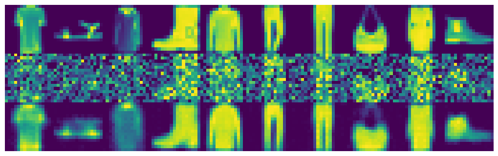 From top to bottom: ground truth, input, and output, with 50% noise.
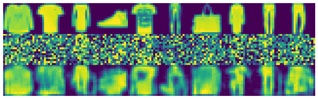 With 75% noise.
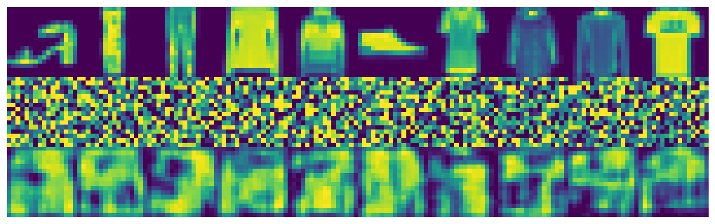 100% noise. Ground truth is irrelavent.
Diffusion models
Sohl-Dickstein et al. (2015)
Sohl-Dickstein et al. (2015)Sohl-Dickstein, Jascha, Eric A. Weiss, Niru Maheswaranathan, and Surya Ganguli. 2015. “Deep Unsupervised Learning Using Nonequilibrium Thermodynamics.” arXiv:1503.03585 is widely regarded as the conceptual origin of modern diffusion-based generative models. Its central contribution is the introduction of a forward–reverse diffusion framework inspired by nonequilibrium statistical physics. In the forward direction, the authors gradually add noise to real data until all structure is destroyed, producing a tractable, simple distribution. In the reverse direction, they train a neural network to undo this corruption process step by step, reconstructing structured samples from pure noise. This idea—slowly destroying structure and then learning to reverse the destruction—became the foundation for all contemporary diffusion models.
Before this work, generative modeling faced a major tension between flexibility and tractability. Flexible models such as energy-based methods were powerful but extremely difficult to train or sample from, while more tractable models lacked expressive capacity. Sohl-Dickstein and colleagues showed that a diffusion process could achieve both. It provided a mathematically principled generative mechanism while preserving stability and avoiding adversarial dynamics, which were major challenges in GAN-based approaches of the time. The paper demonstrated that very deep generative processes with thousands of steps could be trained efficiently and robustly, something that had not been feasible in earlier frameworks.
In historical context, the paper represents a pivotal shift. Published during the period when GANs were gaining attention but suffered from instability and mode collapse, it offered a reliable, probabilistic, and theoretically grounded alternative. Although it did not attract the same immediate popularity at the time, its influence has grown enormously as diffusion models rose to prominence beginning in 2020. Today, nearly every diffusion model implementation traces its core mechanism back to the framework introduced in this work.
In summary, the significance of this paper lies in its foundational insight: that complex data distributions can be modeled by gradually erasing structure through diffusion and learning a neural process that reverses this destruction. This simple but profound idea reshaped generative modeling and underpins much of the current state-of-the-art in AI image, audio, and video generation.
2014 — GANs Introduced. Ian et al. stablished adversarial training, becoming the baseline competitor for diffusion models.Goodfellow, Ian, et al. 2014. “Generative Adversarial Nets.” Advances in Neural Information Processing Systems. Available at arXiv:1406.2661
2015 — Diffusion Framework Introduced. Sohl-Dickstein et al. introduce the forward–reverse diffusion process, laying the foundation for modern diffusion models.Sohl-Dickstein, Jascha, et al. 2015. “Deep Unsupervised Learning Using Nonequilibrium Thermodynamics.” arXiv:1503.03585
2019 — Modern Score Matching. Song & Ermon revive and scale up score matching as a method for generative modeling, directly connecting it to diffusion.Song, Yang, and Stefano Ermon. 2019. “Generative Modeling by Estimating Gradients of the Data Distribution.” NeurIPS
2020 — Score-Based SDE Models. Song & Ermon again propose a unified, continuous-time framework connecting diffusion and stochastic differential equations (SDEs).Song, Yang, and Stefano Ermon. 2020. “Score-Based Generative Modeling through Stochastic Differential Equations.” ICLR
2020 — DDIM: Deterministic Sampling for Diffusion Models. Song et al. introduce Denoising Diffusion Implicit Models (DDIM), which provide a faster, non-Markovian, and deterministic sampling process, significantly speeding up diffusion model inference while maintaining high sample quality.Song, Jiaming, Chenlin Meng, and Stefano Ermon. 2020. “Denoising Diffusion Implicit Models.” ICLR
2021 — Improved DDPM. Nichol & Dhariwal increase sampling speed and sample quality via improved noise schedules.Nichol, Alex, and Prafulla Dhariwal. 2021. “Improved Denoising Diffusion Probabilistic Models.” ICML
2022 — Latent Diffusion → Stable Diffusion. Rombach et al. enable high-resolution image synthesis using latent-space diffusion, making text-to-image models dramatically more compute-efficient.Rombach, Robin, et al. 2022. “High-Resolution Image Synthesis with Latent Diffusion Models.” CVPR
2022 — Classifier-Free Diffusion Guidance. Jonathan Ho & Tim Salimans introduce classifier-free guidance, allowing diffusion models to use conditional information (such as text) for sample generation without a separate classifier network—dramatically improving image quality and controllability in conditional diffusion models.Ho, Jonathan, and Tim Salimans. 2022. “Classifier-Free Diffusion Guidance.” NeurIPS Workshop
2022 — Imagen. Saharia et al. leverage large language model conditioning for photorealistic text-to-image diffusion, rivaling and surpassing GANs in image quality.Saharia, Chitwan, et al. 2022. “Photorealistic Text-to-Image Diffusion Models with Deep Language Understanding.” arXiv:2205.11487
2023 — ControlNet. Zhang & Agrawala introduce a method to condition diffusion models on external spatial structure, such as pose or edges, greatly expanding controllability.Zhang, Lvmin, and Maneesh Agrawala. 2023. “Adding Conditional Control to Text-to-Image Diffusion Models.” arXiv:2302.05543
2023 — Consistency Models. Song et al. propose an alternative to diffusion (“consistency models”), enabling dramatically faster sampling (down to a few or even one step).Song, Yang, et al. 2023. “Consistency Models.” arXiv:2303.01469
2024 — Rectified Flow Transformers (RFT). Esser et al. demonstrate that scaling Rectified Flow Transformers enables high-resolution image synthesis, surpassing previous approaches in photorealism and sample diversity.Esser et al. 2024. “Scaling Rectified Flow Transformers for High-Resolution Image Synthesis.” arXiv:2404.14289
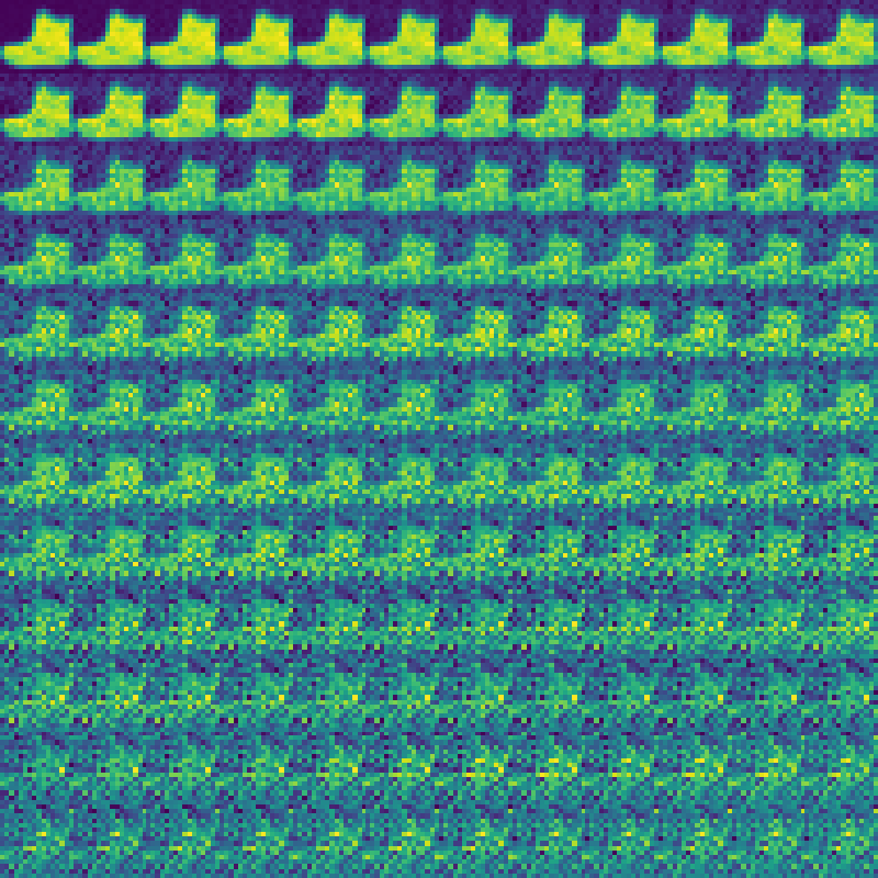
Let \(x_0\) denote data drawn from the true data distribution \(q_0(x)\). The forward diffusion is defined as a Markov chain that progressively increases entropy by adding small amounts of noise at each step. Formally, the forward chain is written as
\[q(x_1, \ldots, x_T \mid x_0) = \prod_{t=1}^T q_t(x_t \mid x_{t-1}),\]where the transition kernels \(q_t(x_t \mid x_{t-1})\) are chosen so that after \(T\) steps the distribution becomes nearly isotropic Gaussian noise. A simple and important example of such a process is Gaussian diffusion, given by
\[q_t(x_t \mid x_{t-1}) = \mathcal{N}(x_t; \sqrt{1-\beta_t}\, x_{t-1}, \beta_t I),\]where \(0 < \beta_t \ll 1\) controls the noise injection rate. After many steps, this process transforms any complex distribution into something close to \(\mathcal{N}(0, I)\), ensuring that sampling from the terminal state is trivial.
plt.figure(figsize=(8, 8))
x_0 = data[0][0].to(device)  # Initial image
x_t = x_0  # Set up recursion
xs = []  # Store x_t for each T to see change

for t in range(T):
    noise = torch.randn_like(x_t)
    x_t = torch.sqrt(1 - B[t]) * x_t + torch.sqrt(B[t]) * noise  # sample from q(x_t|x_t-1)
    img = torch.squeeze(x_t).cpu()
    xs.append(img)
    ax = plt.subplot(nrows, ncols, t + 1)
    ax.axis("off")
    plt.imshow(img)
plt.savefig("forward_diffusion.png", bbox_inches="tight")
The generative model is the reverse-time Markov chain, parameterized by a neural network. Starting from \(x_T \sim \mathcal{N}(0, I)\), the model reconstructs structure by sampling from learned reverse transitions \(p_\theta(x_{t-1} \mid x_t)\). The joint generative distribution is
\[p_\theta(x_{0:T}) = p(x_T) \prod_{t=1}^T p_\theta(x_{t-1} \mid x_t),\]with \(p(x_T) = \mathcal{N}(0, I)\).
revealing that the reverse dynamics depend on the score function
\[\nabla_{x_t} \log q(x).\]This is one of the earliest formulations linking diffusion models to score matching, a connection later exploited by Song & Ermon (2019–2020).
Training is achieved by minimizing the KL divergence between the true forward trajectory distribution and the model’s reverse trajectory distribution:
\[\theta^* = \arg\min_\theta D_{\mathrm{KL}}(q(x_{0:T}) \,\|\, p_\theta(x_{0:T})).\]Expanding this KL divergence yields a sum of local KL divergences between true and learned reverse kernels:
\[L(\theta) = \sum_{t=1}^T \mathbb{E}_{q(x_{t-1}, x_t)} \Big[ D_{\mathrm{KL}} \big( q(x_{t-1} \mid x_t) \;\|\; p_\theta(x_{t-1} \mid x_t) \big) \Big].\]Thus the model is trained to match each reverse transition step individually. This decomposition produces a numerically stable learning procedure, and because each step involves only simple Gaussian distributions, optimization avoids the difficulties seen in adversarial training.
Sampling consists of drawing a noise vector \(x_T \sim \mathcal{N}(0, I)\) and iteratively applying the learned reverse transitions:
\[x_{t-1} \sim p_\theta(x_{t-1} \mid x_t), \quad t = T, T-1, \ldots, 1.\]Each small step gradually removes noise and restores increasing amounts of structure, analogous to annealing a physical system back from high entropy into a low-entropy, structured configuration.
Conceptually, the contribution of this paper is immense: it introduces the idea that deep generative modeling can be performed by learning to reverse a gradual diffusion process that destroys structure in data. This single insight directly enabled later breakthroughs, such as DDPMs (Ho et al. 2020), score-based SDE models (Song & Ermon 2020), and latent diffusion (Rombach et al. 2022), which collectively power modern generative systems like Stable Diffusion, Imagen, DALL·E, and Sora. The thermodynamic framing offered by Sohl-Dickstein et al. provided the theoretical starting point for the entire diffusion revolution.
Ho et al. (2020)
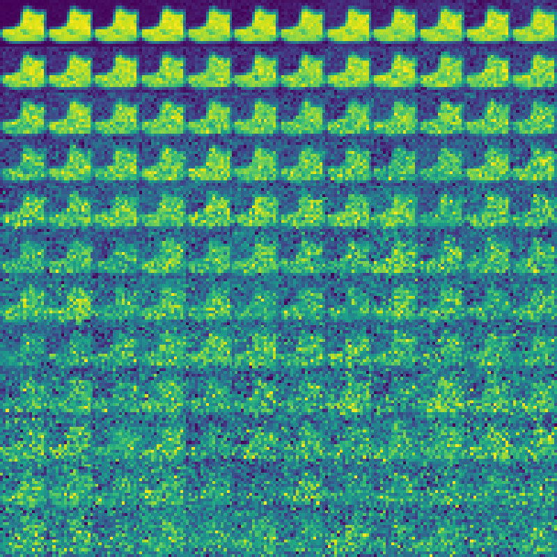
Denoising Diffusion Probabilistic ModelHo, Jonathan, Ajay Jain, and Pieter Abbeel. 2020. “Denoising Diffusion Probabilistic Models.” arXiv:2006.11239 (DDPM, Ho et al., 2020) introduced a set of breakthroughs that solved these issues and made diffusion models practical. It dramatically simplified and improved diffusion models by altering both the parameterization of the reverse transitions and the training objective. Their most important innovation was reparameterizing the reverse mean in terms of the noise added during the forward process, enabling the network to predict \(\epsilon\) rather than the score or the reverse mean. Using the closed-form forward diffusion
\[x_t = \sqrt{\bar{\alpha}_t}\, x_0 + \sqrt{1 - \bar{\alpha}_t}\, \epsilon,\quad \epsilon \sim \mathcal{N}(0, I),\]they showed that the true reverse mean can be written as
\[\mu_\theta(x_t, t) = \frac{1}{\sqrt{\alpha_t}}\, \left(x_t - \frac{\beta_t}{\sqrt{1 - \bar{\alpha}_t}}\, \epsilon_\theta(x_t, t) \right).\]where the forward-noising process is given by
\[q(x_t \mid x_0) = \mathcal{N}\big(x_t; \, \sqrt{\bar{\alpha}_t}\, x_0,\; (1-\bar{\alpha}_t)I\big).\]a = 1. - B
a_bar = torch.cumprod(a, dim=0)
sqrt_a_bar = torch.sqrt(a_bar) # Mean Coefficient
sqrt_one_minus_a_bar = torch.sqrt(1 - a_bar) # St. Dev. Coefficient
def q(x_0, t):
"""
Samples a new image from q
Returns the noise applied to an image at timestep t
x_0: the original image
t: timestep
"""
t = t.int()
noise = torch.randn_like(x_0)
sqrt_a_bar_t = sqrt_a_bar[t, None, None, None]
sqrt_one_minus_a_bar_t = sqrt_one_minus_a_bar[t, None, None, None]
x_t = sqrt_a_bar_t * x_0 + sqrt_one_minus_a_bar_t * noise
return x_t, noise
plt.figure(figsize=(8, 8))
xs = []
for t in range(T):
t_tenser = torch.Tensor([t]).type(torch.int64)
x_t, _ = q(x_0, t_tenser)
img = torch.squeeze(x_t).cpu()
xs.append(img)
ax = plt.subplot(nrows, ncols, t + 1)
ax.set_xticks([])
ax.set_yticks([])
ax.set_frame_on(False)
plt.imshow(img)
plt.subplots_adjust(left=0, right=1, top=1, bottom=0, wspace=0, hspace=0)
plt.savefig("forward_diffusion_skip.png", bbox_inches="tight", pad_inches=0)
Replacing direct score estimation with \(\epsilon\)-prediction dramatically simplifies training and is far more stable. This led to the simple MSE loss
\[L_{\textrm{simple}} = \mathbb{E} \left[ \|\epsilon - \epsilon_\theta(x_t, t)\|^2 \right],\]which outperformed the variational objective used by Sohl-Dickstein et al. and became the standard for all modern diffusion systems (Stable Diffusion, Imagen, etc.).
Another improvement was the introduction of carefully designed variance schedules \(\beta_t\), which avoid the degeneracies and optimization instabilities present in the 2015 model. DDPMs also introduced the idea of fixed or learned variances for the reverse Gaussian
\[p_\theta(x_{t-1} \mid x_t) = \mathcal{N}(x_{t-1};\, \mu_\theta(x_t, t),\, \sigma_t^2 I),\]and found that simply fixing \(\sigma_t^2\) to match the forward process was surprisingly effective. This replaced the complex energy-based interpretations in the original work with a tractable likelihood-based latent-variable model.
sqrt_a_inv = torch.sqrt(1 / a)
pred_noise_coeff = (1 - a) / torch.sqrt(1 - a_bar)

@torch.no_grad()
def reverse_q(x_t, t, e_t):
    t = torch.squeeze(t[0].int())  # All t values should be the same
    pred_noise_coeff_t = pred_noise_coeff[t]
    sqrt_a_inv_t = sqrt_a_inv[t]
    u_t = sqrt_a_inv_t * (x_t - pred_noise_coeff_t * e_t)
    if t == 0:
        return u_t  # Reverse diffusion complete!
    else:
        B_t = B[t-1]
        new_noise = torch.randn_like(x_t)
        return u_t + torch.sqrt(B_t) * new_noise

@torch.no_grad()
def sample_images(ncols, figsize=(8,8)):
    plt.figure(figsize=figsize)
    plt.axis("off")
    hidden_rows = T / ncols

    # Noise to generate images from
    x_t = torch.randn((1, IMG_CH, IMG_SIZE, IMG_SIZE), device=device)

    # Go from T to 0 removing and adding noise until t = 0
    plot_number = 1
    for i in range(0, T)[::-1]:
        t = torch.full((1,), i, device=device)
        e_t = model(x_t, t)  # Predicted noise
        x_t = reverse_q(x_t, t, e_t)
        if i % hidden_rows == 0:
            ax = plt.subplot(1, ncols+1, plot_number)
            ax.axis('off')
            other_utils.show_tensor_image(x_t.detach().cpu())
            plot_number += 1
    plt.show()
Most importantly, DDPM demonstrated that diffusion models can outperform GANs without adversarial training. On CIFAR-10, they achieved state-of-the-art sample quality (FID = 3.17), whereas the 2015 model had shown only conceptual promise but not competitive performance. DDPM also introduced progressive denoising as a generative decoding process, making the model interpretable and setting the stage for latent diffusion (Rombach 2022) and diffusion transformers (2024–2025). DDPM took the elegant but impractical diffusion formulation of Sohl-Dickstein et al. (2015) and introduced the mathematical simplifications, optimization strategies, and noise-prediction parameterization that turned diffusion into a dominant generative modeling framework.
class DownBlock(nn.Module):
    def __init__(self, in_chs, out_chs):
        kernel_size = 3
        stride = 1
        padding = 1

        super().__init__()
        layers = [
            nn.Conv2d(in_chs, out_chs, kernel_size, stride, padding),
            nn.BatchNorm2d(out_chs),
            nn.ReLU(),
            nn.Conv2d(out_chs, out_chs, kernel_size, stride, padding),
            nn.BatchNorm2d(out_chs),
            nn.ReLU(),
            nn.MaxPool2d(2)
        ]
        self.model = nn.Sequential(*layers)

    def forward(self, x):
        return self.model(x)

class UpBlock(nn.Module):
    def __init__(self, in_chs, out_chs):
        # Convolution variables
        kernel_size = 3
        stride = 1
        padding = 1

        # Transpose variables
        strideT = 2
        out_paddingT = 1

        super().__init__()
        # 2 * in_chs for concatenated skip connection
        layers = [
            nn.ConvTranspose2d(2 * in_chs, out_chs, kernel_size, strideT, padding, out_paddingT),
            nn.BatchNorm2d(out_chs),
            nn.ReLU(),
            nn.Conv2d(out_chs, out_chs, kernel_size, stride, padding),
            nn.BatchNorm2d(out_chs),
            nn.ReLU()
        ]
        self.model = nn.Sequential(*layers)

    def forward(self, x, skip):
        x = torch.cat((x, skip), 1)
        x = self.model(x)
        return x

class UNet(nn.Module):
    def __init__(self):
        super().__init__()
        img_chs = IMG_CH
        down_chs = (16, 32, 64)
        up_chs = down_chs[::-1]  # Reverse of the down channels
        latent_image_size = IMG_SIZE // 4 # 2 ** (len(down_chs) - 1)
        t_dim = 1 # New

        # Inital convolution
        self.down0 = nn.Sequential(
            nn.Conv2d(img_chs, down_chs[0], 3, padding=1),
            nn.BatchNorm2d(down_chs[0]),
            nn.ReLU()
        )

        # Downsample
        self.down1 = DownBlock(down_chs[0], down_chs[1])
        self.down2 = DownBlock(down_chs[1], down_chs[2])
        self.to_vec = nn.Sequential(nn.Flatten(), nn.ReLU())

        # Embeddings
        self.dense_emb = nn.Sequential(
            nn.Linear(down_chs[2]*latent_image_size**2, down_chs[1]),
            nn.ReLU(),
            nn.Linear(down_chs[1], down_chs[1]),
            nn.ReLU(),
            nn.Linear(down_chs[1], down_chs[2]*latent_image_size**2),
            nn.ReLU()
        )
        self.temb_1 = EmbedBlock(t_dim, up_chs[0])  # New
        self.temb_2 = EmbedBlock(t_dim, up_chs[1])  # New

        # Upsample
        self.up0 = nn.Sequential(
            nn.Unflatten(1, (up_chs[0], latent_image_size, latent_image_size)),
            nn.Conv2d(up_chs[0], up_chs[0], 3, padding=1),
            nn.BatchNorm2d(up_chs[0]),
            nn.ReLU(),
        )
        self.up1 = UpBlock(up_chs[0], up_chs[1])
        self.up2 = UpBlock(up_chs[1], up_chs[2])

        # Match output channels
        self.out = nn.Sequential(
            nn.Conv2d(up_chs[-1], up_chs[-1], 3, 1, 1),
            nn.BatchNorm2d(up_chs[-1]),
            nn.ReLU(),
            nn.Conv2d(up_chs[-1], img_chs, 3, 1, 1)
        )

    def forward(self, x, t):
        # t encodes the diffusion timestep for each image in the batch.
        # Each value in t is an integer in [0, T], representing how much noise has been applied.
        # Here, we scale t from [0, T] to [0, 1], so it can be used as a continuous input,
        # making temporal embeddings easier and consistent.
        t = t.float() / T  # Normalize timestep to [0, 1]

        # Standard U-Net forward path downsampling
        down0 = self.down0(x)
        down1 = self.down1(down0)
        down2 = self.down2(down1)
        latent_vec = self.to_vec(down2)

        # Project the latent representation and inject timestep embedding at multiple layers
        latent_vec = self.dense_emb(latent_vec)
        temb_1 = self.temb_1(t)  # Temporal embedding injected after dense_emb, affects up0->up1
        temb_2 = self.temb_2(t)  # Temporal embedding injected later in the decoder (up1->up2)

        up0 = self.up0(latent_vec)
        # Add temporal embeddings to feature maps during upsampling to inform the model how much denoising to do
        up1 = self.up1(up0 + temb_1, down2)
        up2 = self.up2(up1 + temb_2, down1)
        return self.out(up2)

model = UNet()
print("Num params: ", sum(p.numel() for p in model.parameters()))
model = torch.compile(UNet().to(device))
The key mechanism enabling denoising is that diffusion models learn the score function, i.e., the gradient of the log probability density of the data at different noise levels:
\[\nabla_{x_t} \log q(x_t \mid x_0)\]Sohl-Dickstein et al. (2015) show that the reverse diffusion process is a discretized form of score-based denoising, since reversing a diffusion corresponds to following the gradient flow of increasing data likelihood. Ho et al. (2020)’s noise-prediction formulation effectively teaches the network to estimate the noise component of a partially corrupted sample. Since:
\[x_0 = \frac{1}{\sqrt{\bar{\alpha}_t}} \left( x_t - \sqrt{1-\bar{\alpha}_t} \, \epsilon \right)\]predicting \(\epsilon\) gives an immediate estimator for a cleaner sample. Each reverse step removes only a small amount of noise—corresponding to the noise injected in the forward process—making the denoising task decomposed and easier. Over hundreds of steps, these local denoising transitions form a coherent global process that reconstructs the data distribution from pure Gaussian noise.
def get_loss(model, x_0, t):
    x_noisy, noise = q(x_0, t)
    noise_pred = model(x_noisy, t)
    return F.mse_loss(noise, noise_pred)

optimizer = Adam(model.parameters(), lr=0.001)
epochs = 3
ncols = 15  # Should evenly divide T

model.train()
for epoch in range(epochs):
    for step, batch in enumerate(dataloader):
        optimizer.zero_grad()

        t = torch.randint(0, T, (BATCH_SIZE,), device=device)
        x = batch[0].to(device)
        loss = get_loss(model, x, t)
        loss.backward()
        optimizer.step()

        if epoch % 1 == 0 and step % 100 == 0:
            print(f"Epoch {epoch} | Step {step:03d} | Loss: {loss.item()} ")
Epoch 0 | Step 000 | Loss: 1.1313930749893188
Epoch 0 | Step 100 | Loss: 0.4029200077056885
Epoch 0 | Step 200 | Loss: 0.33985692262649536
Epoch 0 | Step 300 | Loss: 0.25899502635002136
Epoch 0 | Step 400 | Loss: 0.22377942502498627
Epoch 0 | Step 500 | Loss: 0.24339041113853455
Epoch 1 | Step 000 | Loss: 0.24507106840610504
Epoch 1 | Step 100 | Loss: 0.22035978734493256
Epoch 1 | Step 200 | Loss: 0.21430765092372894
Epoch 1 | Step 300 | Loss: 0.19102375209331512
Epoch 1 | Step 400 | Loss: 0.1935332864522934
Epoch 1 | Step 500 | Loss: 0.19755685329437256
Epoch 2 | Step 000 | Loss: 0.1752050220966339
Epoch 2 | Step 100 | Loss: 0.1929396092891693
Epoch 2 | Step 200 | Loss: 0.1861971616744995
Epoch 2 | Step 300 | Loss: 0.17246274650096893
Epoch 2 | Step 400 | Loss: 0.1772589087486267
Epoch 2 | Step 500 | Loss: 0.17791837453842163