Markov processes and Kolmogorov equations
Jan 1, 2026
Diffusion Project aims to deeply understand diffusion models by tracing their roots in Markov processes and showing how these models connect statistical physics, quantum mechanics, and modern machine learning. The focus is on how geometric and algebraic concepts—such as symmetries, invariants, and representations—govern how information spreads, randomness evolves, and patterns emerge in both physical and computational systems.
Gaussian everything
Brownian motion is not just a probabilistic model but a fundamental natural phenomenon.Nelson, Edward. Dynamical Theories of Brownian Motion. Princeton University Press, 1967. Gaussianity needs explanation, not assumption. The only possible continuous-time, symmetric, small-step random motion on the real line is Brownian motion (or trivial motion).
(Theorem 5.1) Let \(p^t,\; 0 \le t < \infty,\) be a family of probability measures on the real line \(\mathbb{R}\) such that
- (indepdence) \(p^t * p^s = p^{t+s}, \; 0 \le t,s < \infty,\) where \(*\) denotes convolution;
- (small-jump/locality condition) for each \(\varepsilon > 0\), \(p^t\bigl(\{x : |x| \ge \varepsilon\}\bigr) = o(t),\) \(t \to 0,\) and
- (symmetric) for each \(t>0\), \(p^t\) is invariant under the transformation \(x \mapsto -x\).
Then either \(p^t = \delta\) for all \(t \ge 0\) or there is a \(D>0\) such that, for all \(t>0\), \(p^t\) has the density
\[p(t,x) = \frac{1}{\sqrt{4\pi D t}} e^{-x^2/(4Dt)},\]so that \(p\) satisfies the diffusion equation
\[\frac{\partial p}{\partial t} = D\,\frac{\partial^2 p}{\partial x^2}, \; t>0.\]
Measures by construction don’t see locality: you can add spikes, move tiny mass around, and hide pathologies at small scales without changing the measure. Even very different measures can look almost the same (with same mean and variance). What distributions can appear as limits of many convolutions of very small, nearly trivial distributions? Gaussian. Convolution converts adding independent increments to kernel actions. It smooths out microscopic structure and amplifies only low-order moments, so limits of convolutions are rigid. Gaussians dominate and diffusion (Laplacians) appears. Diffusion is the PDE encoding of a convolution limit.
Measures are too flexible. The semigroup condition still leaves many degrees of freedom out. Operator however is rigid. It gives a massive information upgrade by tracking how the process acts on every test function:
\[(P^t f)(x) = \int f(x + y)\, p^t(dy).\]It describes how observables evolve. Random variables being added turn into measures convoluted, into operators composed. We can do even better. Introduce the infinitesimal generator \(A.\) The entire semigroup is encoded in one operator—if you classify generators, you classify processes:
\[\begin{align*} A f &= \lim_{t \to 0^+} \frac{P^t f - f}{t} \\ &= \frac{1}{t} \left( f'(x)\int y\,p^t(dy) + \frac{1}{2} f''(x)\int y^2\,p^t(dy) + \text{smaller terms} \right)\\ & = D f''(x) \end{align*}\]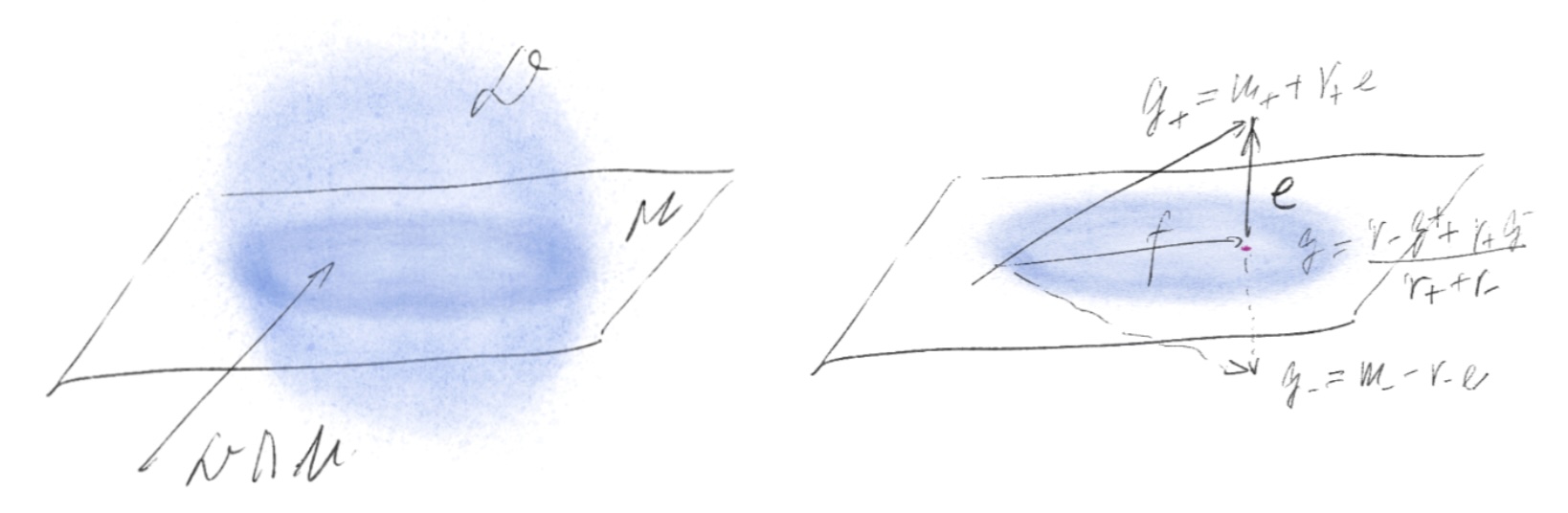 Dense approximations can be made exact on finite dimensions. Functions can be approximated by elements in the generator’s domain $$\mathcal{D}$$—qua a dense convex linear subspace—while preserving values and derivatives at a point, which is essential for identifying the generator as a second-order diffusion operator. Given a continuous linear function $$u\in\mathcal{X}^*$$ and $$\mathcal{M} =\ker u$$ is the desired subspace with "good" points. Choose $$e\in\mathcal{X}$$ with $$u(e)=1$$ yields the decomposition: $$\mathcal{X} = \mathcal{M}\oplus\mathbb{R}e$$. For any $$f \in \mathcal{X}$$, dense gives you an approximation $$g \in \mathcal{D}$$. Only need to constrant $$g$$ to $$\mathcal{M}$$.
A measure can hide pathologies at scale. But the generator sees: first-order effects (drift, killed by symmetry); second-order effects (diffusion); and jump intensities (residual, killed by locality). Measures allow infinitely many microscopic perturbations that do not affect macroscopic properties; infinitesimal generators collapse these perturbations into finitely many coefficients.
Kolmogorov equations
One word of caution. Probability can feel cursed because a single symbol \(P\) is used everywhere with disambiguation left entirely to context:
- Any Markov process,
- If continuous kernel exisits,
- If time homogeneous,
In the standard (e.g., SDE) treatment, diffusion is taken as an assumption. Following Nelson, however, diffusion emerges naturally from the underlying Markov structure.
(Markov process) Let \((\Omega,\mathcal F,\mathbb P)\) be a probability space, \((\mathcal F_t)_{t \ge 0}\) a filtration on \(\Omega\), \((E,\mathcal E)\) a measurable space, and \((X_t)_{t \ge 0}\) an \(E\)-valued stochastic process such that \(X_t\) is \(\mathcal F_t\)-measurable for every \(t \ge 0\).
The process \((X_t)_{t \ge 0}\) is called a Markov process with respect to the filtration \((\mathcal F_t)\) if for all \(t,s \ge 0\) and all bounded \(\mathcal E\)-measurable functions \(f : E \to \mathbb R\),
\[\mathbb E\!\left[ f(X_{t+s}) \mid \mathcal F_t \right] = \mathbb E\!\left[ f(X_{t+s}) \mid X_t \right] \quad \text{a.s.}\]
 The Chapman–Kolmogorov equation expresses the Markov property by factorizing long-time transitions through intermediate states, effectively integrating over intermediate paths.
 (Chapman–Kolmogorov) There exists a family of transition probability kernels \((P_t)_{t \ge 0}\),
\[P_t : E \times \mathcal E \to [0,1],\]such that for all \(t,s \ge 0\) and all \(A \in \mathcal E\),
\[\mathbb P(X_{t+s} \in A \mid \mathcal F_t) = P_s(X_t,A) \quad \text{a.s.}\]and the Chapman–Kolmogorov equation holds:
\[P_{t+s}(x,A) = \int_E P_t(x,dy)\,P_s(y,A).\]
The process \((X_t)_{t \ge 0}\) is called strong Markov if for every stopping time \(\tau\) and every \(s \ge 0\),
\[\mathbb E\!\left[ f(X_{\tau+s}) \mid \mathcal F_\tau \right] = \mathbb E\!\left[ f(X_{\tau+s}) \mid X_\tau \right] \quad \text{a.s.}\]
Functional analysis can be viewed as the natural extension of matrix multiplication to infinite-dimensional spaces. A kernel plays the role of an infinite-dimensional Gram matrix, encoding inner products between functions rather than finite-dimensional vectors:
\[(Gc)_i = \langle v_i, w\rangle \ \text{where}\ w = \sum_{j} c_j\, v_j \ \Longrightarrow\ (Tf)(x) = \int k(x,y)\, f(y)\, dy .\]The Chapman–Kolmogorov equation is the measure-theoretic expression of the semigroup property of transition probability kernels; it follows directly from the Markov property. Brownian motion is the canonical continuous-time Markov process. Brownian motion = Markov + continuous + symmetric + local. Adjointness is clear from matrix multiplication.
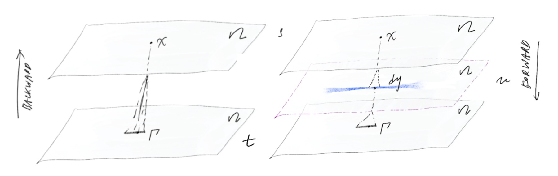
(Kolmogorov backward) Let \(f(x) \in C_b(\mathbb{R})\), and let
\[u(x,s) := \mathbb{E}\!\left(f(X_t)\mid X_s = x\right) = \int f(y)\,P(dy,t\mid x,s),\]with \(t\) fixed. Assume, furthermore, that the functions \(b(x,s)\), \(\Sigma(x,s)\) are smooth in both \(x\) and \(s\). Then \(u(x,s)\) solves the final value problem
\[-\frac{\partial u}{\partial s} = b(x,s)\frac{\partial u}{\partial x} + \frac12\,\Sigma(x,s)\frac{\partial^2 u}{\partial x^2}, \ u(t,x)=f(x), \quad\text{for}\ s \in [0,t].\]
The backward equation is about observables \(u\), which is well-defined for any Markov process. It satisfies
\[-\partial_s u = \mathscr{L} u.\]The forward Kolmogorov equation is always true at the level of measures:
\[\partial_t \mu_t = \mathscr{L}^*\mu_t\]and \(\mathscr{L}^*\) is the adjoint of the generator. The backward equation evolves functions through the semigroup, while the forward equation evolves probability mass, which only becomes a PDE after assuming that mass has a density.
\[\frac{\partial p}{\partial t}(y,t\mid x,s) = -\frac{\partial}{\partial y}\!\left(b(y,t)\,p(y,t\mid x,s)\right) + \frac12\,\frac{\partial^2}{\partial y^2}\!\left(\Sigma(y,t)\,p(y,t\mid x,s)\right),\]and
\[\lim_{t\downarrow s} p(y,t\mid x,s)=\delta(y-x).\]That is, the solution to Fokker-Planck equation provides the kernel. Functions and measures are dual because measures are exactly the linear objects that eat functions and return numbers, and all Kolmogorov/Fokker–Planck theory is just the dynamics of this dual pairing.
Riemmannian geometry, Lie algebra, gauges, and Cohomology
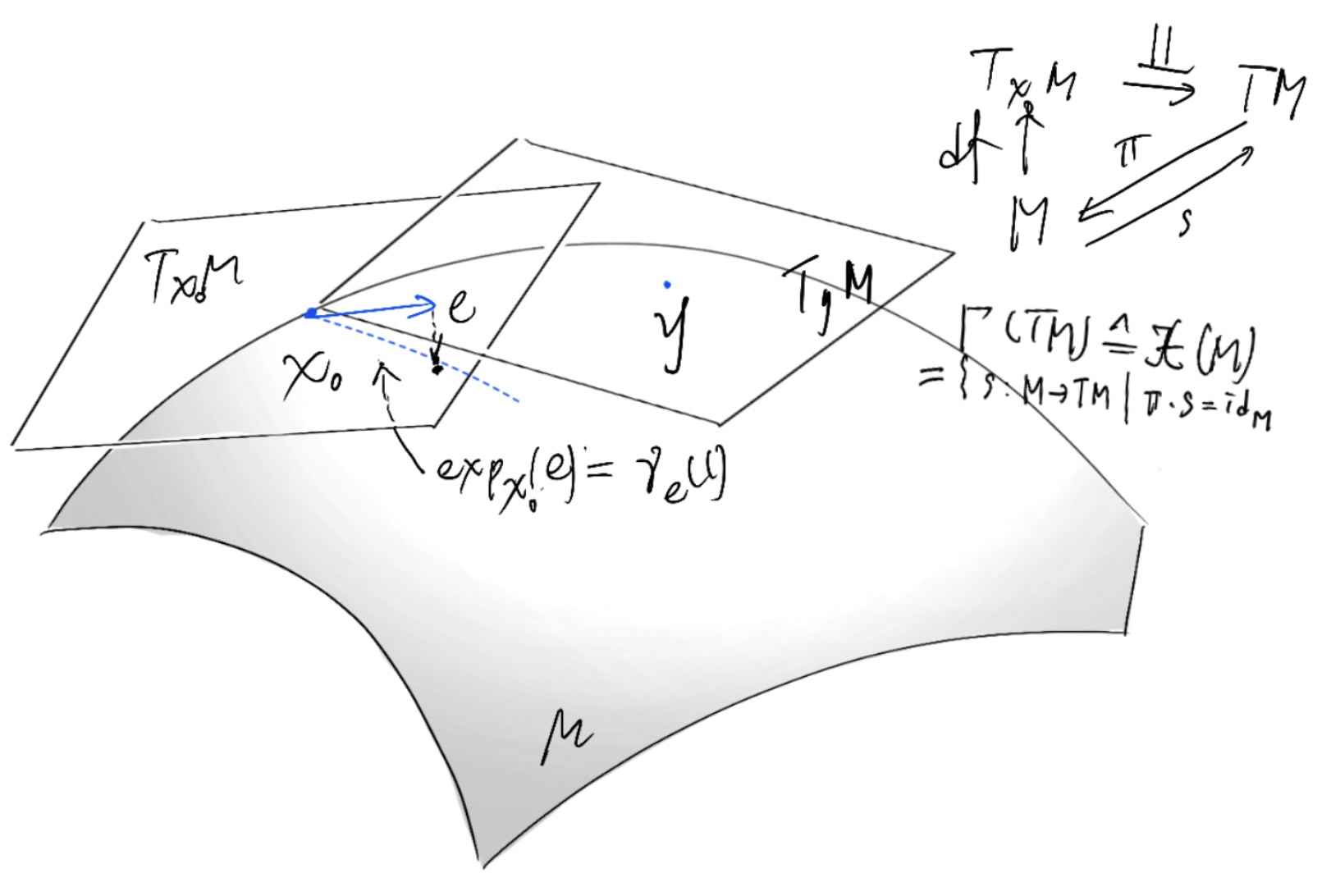 Sections of the tangent bundle are defined fiberwise: vectors for a vector field on \(M\) do not all live in the same vector space. Riemannian geometry exists because tangent vectors live in different fibers with no canonical identification; only transport via a (path-dependent) connection allows comparison, and the obstruction to doing so globally is curvature.
Consider a state manifold \(M\). Diffeomorphisms \(\text{Diff}(\mathcal{M})\) gives an infinite-dimension Lie group. Deterministic ODE \(d_t X_t = u_t(X_t)\) generates a flow \(\phi_t: M\to M\) and \(X_0 \mapsto X_t=\phi_t(X_0)\). You can push forward any probability measure \(p\) on \(M\) according to \(\phi_t\):
\[((\phi_t)_\# p)(A) := p(\phi_t^{-1}(A)),\]which gives the evolution of probability induced by the flow. \(\text{Diff}(\mathcal{M})\) acts transitively on \(\mathcal{P}(\mathcal{M})\), and
\[\mathcal{P}(\mathcal{M}) \cong \text{Diff}(\mathcal{M})/\text{Stab}(p).\]Infinitesimally,
\[\begin{array}{ccc} \mathrm{Diff}(M)\times \mathcal{P}(M) & \xrightarrow{\quad (\phi,\rho)\mapsto \phi_\#\rho \quad } & \mathcal{P}(M) \\ \downarrow\scriptstyle{\mathrm{d}|_{(id,\rho)}} & & \downarrow\scriptstyle{\mathrm{d}|_{\rho}} \\ \mathfrak{X}(M)\times \mathcal{P}(M) & \xrightarrow{\quad (u,\rho)\mapsto -\operatorname{div}(\rho u)\quad } & T_{\rho}\mathcal{P}(M) \end{array}\]The Laplacian term in a diffusion generator is a trivial cocycle in the coadjoint representation of the diffeomorphism Lie algebra, and the score correction is the gauge transformation that removes it.
Sometimes extra terms represent nontrivial cohomology; here the extra term is removable (exact) once you allow state-dependent gauge.
Quantum mechanics
Stochastic mechanics is the classical shadow of quantum mechanics, and Theorem 13 is the statement that noise-induced diffusion is a gauge choice at the level of state evolution, just as different quantum unravelings describe the same mixed state.
Portfolio Management
Active portfolio returns are written as
\[r_t^p = w^\top F r_t^F + w^\top r_t^I,\]where \(w \in \mathbb{R}^N\) denotes active weights, \(F \in \mathbb{R}^{N\times K}\) is the factor exposure matrix, \(r_t^F \in \mathbb{R}^K\) are factor returns, and \(r_t^I \in \mathbb{R}^N\) are idiosyncratic returns. Assuming zero mean returns, factor covariance \(\Sigma \in \mathbb{R}^{K\times K}\), and idiosyncratic covariance \(\Lambda \in \mathbb{R}^{N\times N}\) (typically diagonal), the tracking error is
\[\mathrm{TE}^2 = w^\top F \Sigma F^\top w + w^\top \Lambda w.\]Over a horizon \(t\),
\[r_t^p \sim \mathcal N\!\left(0,\; t\,\mathrm{TE}^2\right).\]Define the state variable
\[X_t := r_t^p.\]Then \(X_t\) satisfies the stochastic differential equation
\[dX_t = \sigma_p\, dW_t, \quad \sigma_p^2 = \mathrm{TE}^2.\]The infinitesimal generator is
\[\mathcal L u(x) = \frac12 \sigma_p^2 \frac{\partial^2 u}{\partial x^2}.\]Rather than modeling the scalar portfolio return directly, model the underlying drivers. Let \(r_t^F \in \mathbb{R}^K\) denote factor returns and \(r_t^I \in \mathbb{R}^N\) denote idiosyncratic returns. In continuous time, assume driftless diffusions
\[dr_t^F = \Sigma^{1/2}\, dW_t^F, \qquad dr_t^I = \Lambda^{1/2}\, dW_t^I,\]where \(W_t^F \in \mathbb{R}^K\) and \(W_t^I \in \mathbb{R}^N\) are independent Brownian motions.
Define the full state vector
\[X_t := \begin{pmatrix} r_t^F\\ r_t^I \end{pmatrix}.\]Then \(X_t\) is a multidimensional time-homogeneous Markov diffusion. The portfolio return is the linear projection
\[r_t^p = w^\top F r_t^F + w^\top r_t^I.\]Since \(X_t\) is Gaussian Markov and \(r_t^p\) is a linear functional of \(X_t\), the portfolio return is again a (scalar) Gaussian Markov diffusion with instantaneous variance
\[\sigma_p^2 = w^\top F \Sigma F^\top w + w^\top \Lambda w.\]Let \(P_t(x,A)\) denote the transition kernel of \(X_t\). The Chapman–Kolmogorov equation is
\[P_{t+s}(x,A) = \int_{\mathbb R} P_t(x,dy)\,P_s(y,A).\]This implies additive variance:
\[\mathrm{Var}(r_{t+s}^p) = \mathrm{Var}(r_t^p) + \mathrm{Var}(r_s^p).\]For an observable \(f\), define
\[u(x,s) = \mathbb E[f(X_t)\mid X_s=x].\]Then
\[-\frac{\partial u}{\partial s} = \mathcal L u = \frac12 \sigma_p^2 \frac{\partial^2 u}{\partial x^2}, \quad u(x,t)=f(x).\]Let \(p(x,t)\) denote the density of \(X_t\). Then
\[\frac{\partial p}{\partial t} = \frac12 \sigma_p^2 \frac{\partial^2 p}{\partial x^2}, \quad p(x,0)=\delta(x).\]The solution is
\[p(x,t) = \mathcal N\!\left(0,\; t\,\sigma_p^2\right).\]The factor risk model determines the generator of the Markov process. Tracking error is the diffusion coefficient, Chapman–Kolmogorov encodes time aggregation of risk, the backward equation propagates expectations, and the forward equation propagates probability mass.
Returns are pairings between a state vector and a weight vector:
\[r_t^{a}\ = \langle w, r_t\rangle, \qquad r_t^{\mathrm{adj}} = \langle w^{\mathrm{adj}}, r_t\rangle,\]where weights define linear functionals acting on the random state. Adjusting the benchmark changes the functional (the weight vector) but not the underlying Markov dynamics of the state. If portfolio weights are predictable and returns follow a continuous-time diffusion, the cumulative active return over $[0,T]$ can be written as \(\int_0^T w_t^\top \, dR_t .\)
Under standard regularity conditions, the Ito isometry implies the exact variance identity
\[\operatorname{Var}\!\left( \int_0^T w_t^\top \, dR_t \right) = \mathbb{E}\!\left[ \int_0^T w_t^\top \, \Sigma_{\mathrm{true}}(t) \, w_t \, dt \right],\]where \(\Sigma_{\mathrm{true}}(t)\) is the instantaneous covariance matrix of returns.